Time Complexity#
Time Complexity is a theoretical measure that quantifies the amount of time an algorithm takes to run as a function of the length of its input (\(n\)). Instead of measuring actual seconds—which change based on hardware, compilers, and processors—time complexity counts the number of elementary operations or code statements executed.
Asymptotic Notations#
Algorithms can perform differently depending on the structure of the input data. We analyze them using three main bounds:
Worst-Case#
Big O notation \(O\) is a mathematical metric used to describe the efficiency and performance of an algorithm. It measures how the execution time or space requirements grow relative to the input size (\(n\)), specially representing the worse-case scenario (upper bound).
Best-Case#
Big Omega notation \(Ω\) defines the asymptotic lower bound of an algorithm’s time complexity. It represents absolute minimum time or steps an algorithm requires to run for large input sizes. In simpler terms, it answers the question: “At the very least, how fast will this algorithm grow?”.
Average-Case#
Big Theta notation \(Θ\) defines a tight asymptotic bound on the execution time of an algorithm. Unlike Big O (which provides a maximum boundary) or Big Omega (which provides a minimum boundary), Big Theta bounds a function from both above and below. This means the algorithm’s actual performance scales precisely at the rate indicated by the bounding function as input size grows toward infinity.
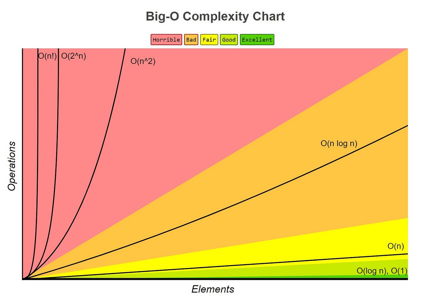
Common Time Complexities#
Ordered by efficiency:
Constant Time \(O(1)\)#
Execution time remains the same regardless of input size.
Common Examples
Accessing an array element by its index.
template <int size>
int constant(int (&array)[size]) {
  return array[0];
}
def constant(array: list[int]) -> int:
  return array[0]
Logarithmic Time \(O(log n)\)#
The problem size is divided by a factor (usually halved) at each step.
Common Examples
int power(int base, int exponent) {
  int result { 1 };
  while (0 < exponent) {
    if (exponent % 2 == 1) {
      result *= base;
    }
    base *= base;
    exponent /= 2;
  }
  return result;
}
def power(base: int, exponent: int) -> int:
  result: int = 1
  while 0 < exponent:
    if exponent % 2 == 1:
      result *= base
    base *= base
    exponent //= 2
  return result
Linear Time \(O(n)\)#
Running time grows in direct proportion to the input size.
Common Examples
A single loop traversing a list.
template <int size>
void linear(int (&array)[size]) {
  for (int element : array) {
    std::cout << element << " ";
  }
}
def linear(array: list[int]) -> None:
  for element in array:
    print(element)
Linearithmic Time \(O(n log n)\)#
Slightly worse than linear, typical for efficient sorting mechanisms.
Common Examples
Merge Sort and Quick Sort
int linearithmic(int size) {
  int count { 0 };
  for (int i = 0; i < size; ++i) {
    int j { size };
    while (1 < j) {
      j /= 2;
      count += 1;
    }
  }
  return count;
}
def linearithmic(size: int) -> int:
  count: int = 0
  for i in range(size):
    j: int = size
    while 1 < j:
      j //= 2
      count += 1
  return count
Quadratic Time \(O(n ^ 2)\)#
Execution time scales non-linearly, squaring the input size growth.
Common Examples
Nested loops, like Bubble Sort
template <int size>
void quadratic(int (&array)[size]) {
  for (int i = 0; i < size; ++i) {
    for (int j = 0; j < size; ++j) {
      std::cout << i << j << std::endl;
    }
  }
}
def quadratic(array: list[int]) -> None:
  for i in array:
    for j in array:
      print(i, j)
Exponential Time \(O(2 ^ n)\)#
Growth doubles with each additional data unit; quickly becomes unrunnable.
Common Examples
Recursive Fibonacci sequence calculations.
int fibonacci(int n) {
  if (n < 2) return n;
  return fibonacci(n - 1) + fibonacci(n - 2);
}
def fibonacci(n: int) -> int:
  if n < 2: return n
  return fibonacci(n - 1) + fibonacci(n - 2)
Factorial Time \(O(n!)\)#
Grows incredibly fast; completely unusable for inputs larger than \(n ≈ 10\).
Common Examples
Generating all permutations of a string, or solving the Traveling Salesperson Problem.
std::vector<std::vector<int>> permutations(std::vector<int> &array) {
  if (array.size() <= 1) return { array };
  std::vector<std::vector<int>> allPermutations;
  for (int i = 0; i < array.size(); ++i) {
    int current { array[i] };
    std::vector<int> remaining;
    remaining.insert(remaining.end(), array.begin(), array.begin() + i);
    remaining.insert(remaining.end(), array.begin() + i + 1, array.end());
    std::vector<std::vector<int>> subpermutations { permutations(remaining) };
    for (int i = 0; i < subpermutations.size(); ++i) {
      std::vector<int> permutation { current };
      permutation.insert(permutation.end(), subpermutations[i].begin(), subpermutations[i].end());
      allPermutations.push_back(permutation);
    }
  }
  return allPermutations;
}
def permutations(array: list[int]) -> list[list[int]]:
  if len(array) <= 1: return [array]
  all_permutations: list[list[int]] = list()
  for i in range(len(array)):
    current: int = array[i]
    remaining: list[int] = array[:i] + array[i + 1:]
    for permutation in permutations(remaining):
      all_permutations.append([current] + permutation)
  return all_permutations
How to Calculate Time Complexity#
To determine the time complexity of a block of code, follow these three practical rules:
- Count the loops.
A single loop running from \(0\) to \(n\) takes \(O(n)\) time.
Two nested loops running up to \(n\) take \(n * n = O(n ^ 2)\) time.
- Drop constant terms.
Big O isolates the overall growth trend. If an algorithm takes \(2n + 5\) operations, drop the multiplier \(2\) and the constant \(5\). The time complexity is simply \(O(n)\).
- Keep only the dominating term.
If a code snippet has one portion taking \(O(n ^ 2)\) and another taking \(O(n)\), the total time formula is \(n ^ 2 + n\). As \(n\) approaches infinity, the \(n\) term becomes insignificant next to \(n ^ 2\). Keep only the largest term: \(O(n ^ 2)\).